Brexit Analysis

Analysis of Leave Share

leave_share - the percent of votes cast in favour of Brexit in each constituency of the UK

Plotting a histogram, a density plot, and the empirical cumulative distribution function of the leave % in all constituencies to get a sense of the distribution of values.

# histogram
ggplot(brexit_results, aes(x = leave_share)) +
  geom_histogram(binwidth = 2.5) +
  labs(title = "Brexist Vote Analysis - Distribution of leave share",
       x = "leave share",
       y = "Number of Constituencies")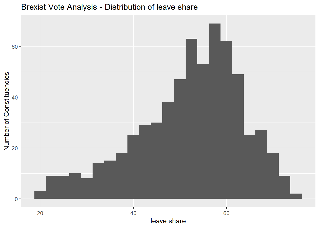

# density plot-- think smoothed histogram
ggplot(brexit_results, aes(x = leave_share)) +
  geom_density() +
  labs(title = "Brexit Vote Analysis - leave share density distribution",
       x = "leave share",
       y = "Density")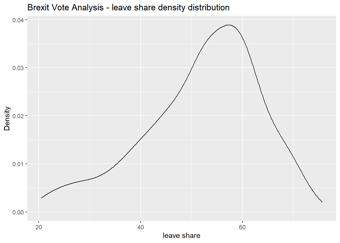

# The empirical cumulative distribution function (ECDF) 
ggplot(brexit_results, aes(x = leave_share)) +
  stat_ecdf(geom = "step", pad = FALSE) +
  scale_y_continuous(labels = scales::percent) +
  labs(title = "Brexit Vote Analysis - leave share ECDF function",
       x = "leave share",
       y = "Cumulative Density of Constituencies")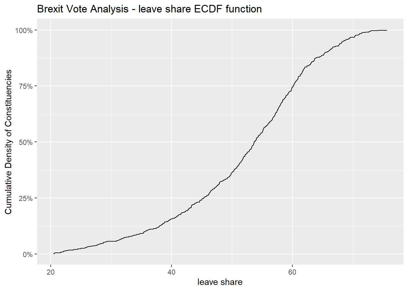   

Leave Share vs Born in UK

Analysing correlation between the % of UK born voters in a constituency vs the % of people who voted in favour of Brexit:

One common explanation for the Brexit outcome was fear of immigration and opposition to the EU’s more open border policy. We first check the or correlation between the proportion of native born residents (born_in_uk) in a constituency and its leave_share.

brexit_results %>% 
  select(leave_share, born_in_uk) %>% 
  cor()

##             leave_share born_in_uk
## leave_share   1.0000000  0.4934295
## born_in_uk    0.4934295  1.0000000

The correlation is almost 0.5, which shows that the two variables are reasonably positively correlated but not very strongly.

To view the data, we also create a scatterplot between these two variables and add the best fit line.

brexit_results %>% 
  ggplot(aes(x = born_in_uk, y = leave_share)) +
  geom_point(alpha=0.3) +
  
  # add a smoothing line, and use method="lm" to get the best straight-line
  geom_smooth(method = "lm") + 
  
  # use a white background and frame the plot with a black box
  theme_bw() +
  labs(title = "Brexit Vote Analysis - Correlation: leave share vs proportion born in UK",
       x = "born in UK",
       y = "leave share") 

## `geom_smooth()` using formula 'y ~ x'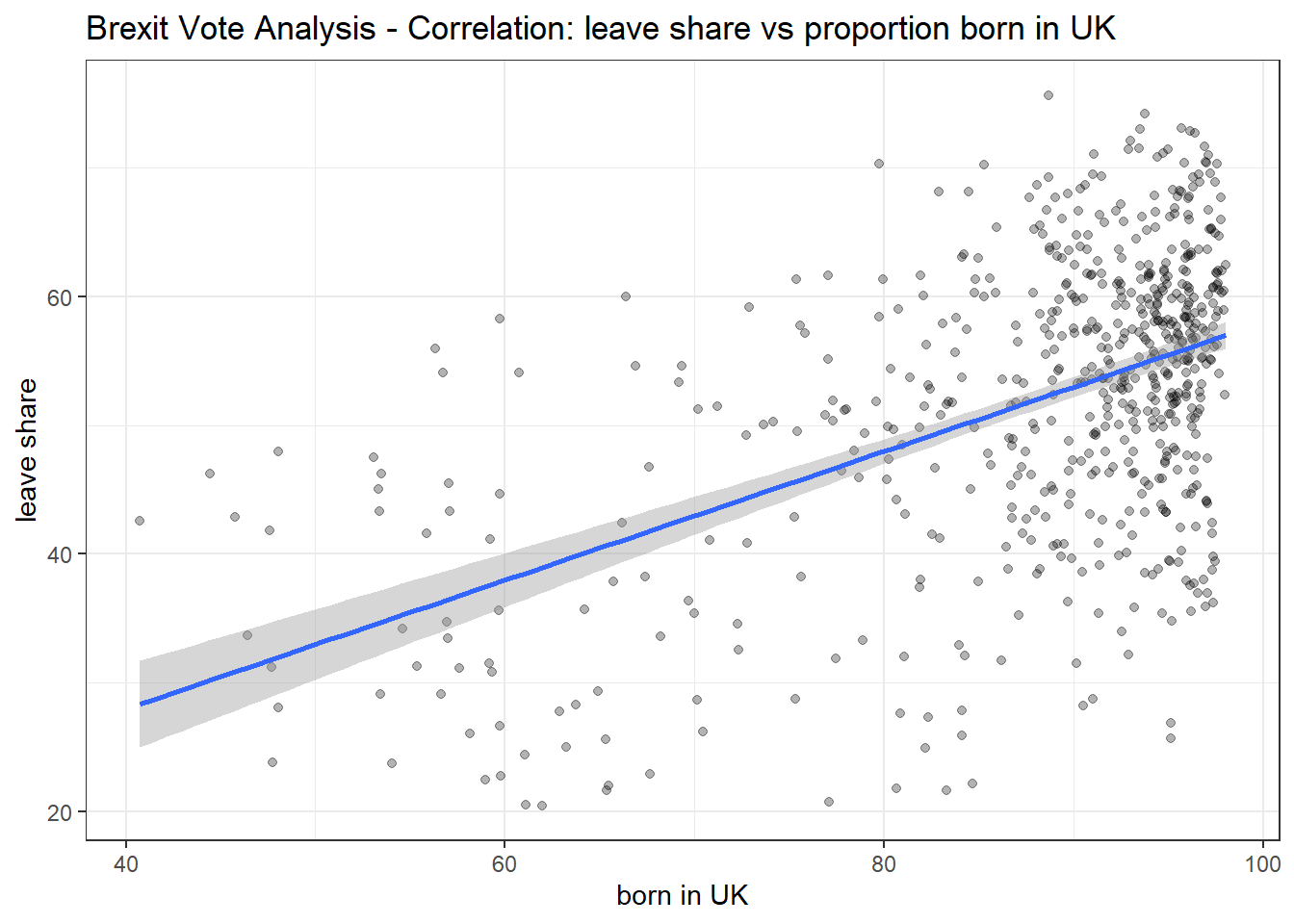

Running a linear regression model to quantify this correlation:

model_uk_leave_share <- lm(leave_share ~ born_in_uk, data= brexit_results)
msummary(model_uk_leave_share)

##             Estimate Std. Error t value Pr(>|t|)    
## (Intercept)  7.97669    3.12104   2.556   0.0108 *  
## born_in_uk   0.50005    0.03512  14.239   <2e-16 ***
## 
## Residual standard error: 9.957 on 630 degrees of freedom
## Multiple R-squared:  0.2435, Adjusted R-squared:  0.2423 
## F-statistic: 202.8 on 1 and 630 DF,  p-value: < 2.2e-16

Taken individually, born_in_uk is a significant variable in predicting the leave share of a constituency and explains about 24% of the variations in leave share.

General Observations:

Constituencies with higher percentage of people born in the UK seem to show higher support for the exit. While there are few exceptions, places with over 85% UK-born population tend to have leave shares of above 40%, concentrating around 58% and the confidence interval of leave shares decreases with an increase in local residents. A large proportion of constituencies also happen to have high percentage of UK-born residents with possible apprehension towards a more competitive job market, loss of local opportunities to potential immigrants and impact on local lifestyle and culture from migration.

To be noted however, that we have not taken into account any other contributing factor towards leave_share and this correlation only considers the effect of UK-born resident % in isolation.

Leave Share vs Political Affiliation

Considering the correlation between the political party affiliation of the public and their support/ opposition of Brexit.

Visualization - Collaborated with: Emma Clark, Alice Chen, Yuqiao Leng and Joël Merki (LBS MAM23)

# create a list of hex color codes for political parties
color_list=c("#0087DC","#E4003B","#FFEEAA","#6D3177")

# Renaming political parties and pivotting longer
brexit_results_longer <- brexit_results %>% 
  rename("Conservative" = "con_2015",
         "Labour" = "lab_2015",
         "Lib Dems" = "ld_2015",
         "UKIP" = "ukip_2015"
         ) %>% 
  pivot_longer(c(2:5), names_to="party", values_to = "seat_percent")
  
# Plotting results
ggplot(brexit_results_longer, 
  aes(x = seat_percent, y = leave_share, group = party)) +
  geom_point(aes(color = factor(party))) +
  geom_smooth(aes(color = factor(party)),method="lm") +
  scale_color_manual(values = color_list) +
  theme_bw() +
  theme(legend.title=element_blank()) +
  theme(legend.position = "bottom") +
  labs(title = "How political affiliation translated to Brexit Voting") +
  xlab("Party % in the UK 2015 general election") +
  ylab("Leave % in the 2016 Brexit referendum")

## `geom_smooth()` using formula 'y ~ x'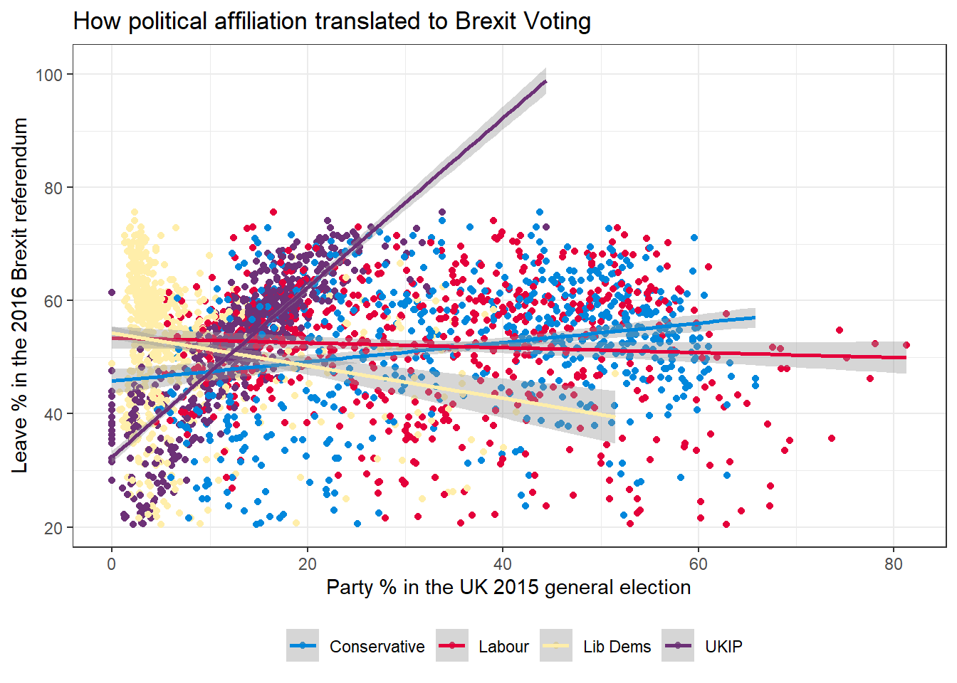

Running a linear regression model and ggpairs plot to view this correlation:

model_political <- lm(leave_share ~ con_2015+lab_2015+ld_2015+ukip_2015, 
                      data= brexit_results)
msummary(model_political)

##             Estimate Std. Error t value Pr(>|t|)    
## (Intercept) 36.68505    1.56185  23.488  < 2e-16 ***
## con_2015    -0.01778    0.02128  -0.836 0.403662    
## lab_2015    -0.07003    0.02264  -3.094 0.002066 ** 
## ld_2015     -0.12830    0.03448  -3.721 0.000216 ***
## ukip_2015    1.47191    0.03916  37.589  < 2e-16 ***
## 
## Residual standard error: 6.008 on 627 degrees of freedom
## Multiple R-squared:  0.7258, Adjusted R-squared:  0.7241 
## F-statistic:   415 on 4 and 627 DF,  p-value: < 2.2e-16

ggpairs(brexit_results, columns = c('con_2015','lab_2015','ld_2015','ukip_2015','leave_share'))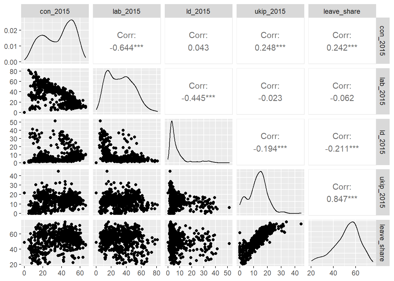

At first glance, the strongest correlation can be observed looking at correlation between UKIP party % and leave %. We can infer that the higher the representation of the UK Independence Party in a county, the higher the votes in favor of leaving the EU. At the same, there seems to be a slight negative correlation between the representation of liberal deomcrats in a county and leave share.

Again, to be noted that this correlation only considers the effect of political party affiliation in isolation.

Other predictors of leave share

ggpairs to view correlation:

ggpairs(brexit_results, columns = c('con_2015','lab_2015','ld_2015','ukip_2015',
                                    'born_in_uk','male','unemployed',
                                    'degree','age_18to24','leave_share'))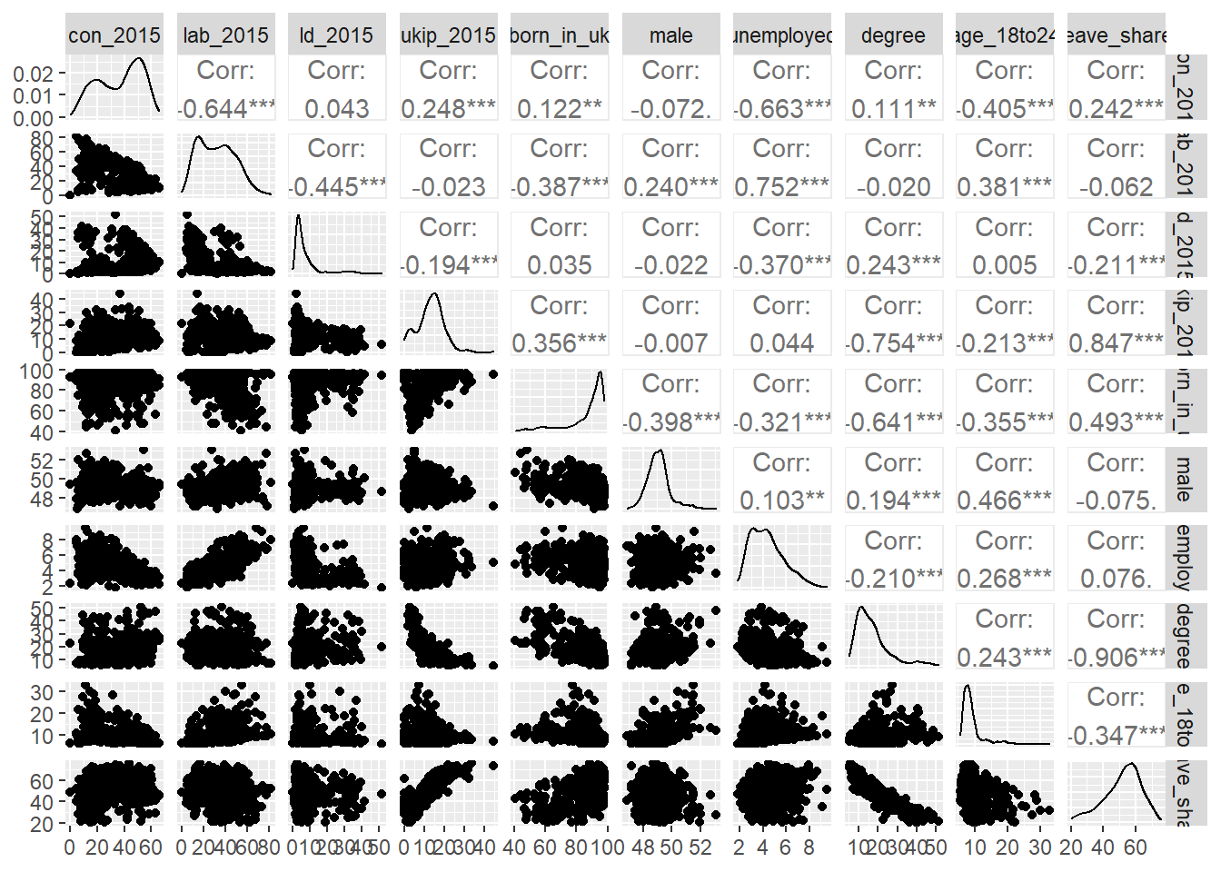

We notice that degree (education level) and affiliation towards the UK Independent Party both show a high correlation to leave share when taken along with all other predictors.

model_leave_all <- lm(leave_share ~ con_2015 + lab_2015 + ld_2015 + ukip_2015 +
                        born_in_uk + male + unemployed + degree + age_18to24, 
                      data= brexit_results)
msummary(model_leave_all)

##              Estimate Std. Error t value Pr(>|t|)    
## (Intercept)  6.090941  11.174471   0.545 0.585917    
## con_2015     0.236923   0.022694  10.440  < 2e-16 ***
## lab_2015     0.129272   0.025187   5.132 3.94e-07 ***
## ld_2015      0.132890   0.027913   4.761 2.45e-06 ***
## ukip_2015    0.786945   0.042635  18.458  < 2e-16 ***
## born_in_uk  -0.007348   0.020737  -0.354 0.723221    
## male         0.743495   0.203906   3.646 0.000291 ***
## unemployed   0.449130   0.189008   2.376 0.017823 *  
## degree      -0.826423   0.030711 -26.909  < 2e-16 ***
## age_18to24  -0.259768   0.047583  -5.459 7.18e-08 ***
## 
## Residual standard error: 3.079 on 563 degrees of freedom
##   (59 observations deleted due to missingness)
## Multiple R-squared:  0.9202, Adjusted R-squared:  0.9189 
## F-statistic: 721.2 on 9 and 563 DF,  p-value: < 2.2e-16

vif(model_leave_all)

##   con_2015   lab_2015    ld_2015  ukip_2015 born_in_uk       male unemployed 
##   7.050112  10.847648   2.967263   3.402759   3.506365   1.514946   4.396018 
##     degree age_18to24 
##   3.973118   1.764195

The VIF of Labour party supporters (lab_2015) is above 10, suggesting multicolleniearity. So we drop that and rerun our model.

model_leave_all2 <- lm(leave_share ~ con_2015 + ld_2015 + ukip_2015 +
                        born_in_uk + male + unemployed + degree + age_18to24, 
                      data= brexit_results)

#Calculate VIF
vif(model_leave_all2)

##   con_2015    ld_2015  ukip_2015 born_in_uk       male unemployed     degree 
##   2.718999   1.318469   2.444450   3.489675   1.512837   3.898942   3.938543 
## age_18to24 
##   1.764052

#Model summary stats
msummary(model_leave_all2)

##             Estimate Std. Error t value Pr(>|t|)    
## (Intercept) 17.83154   11.18086   1.595 0.111311    
## con_2015     0.14563    0.01441  10.108  < 2e-16 ***
## ld_2015      0.02610    0.01902   1.372 0.170534    
## ukip_2015    0.67082    0.03694  18.160  < 2e-16 ***
## born_in_uk  -0.01469    0.02115  -0.695 0.487538    
## male         0.70444    0.20829   3.382 0.000769 ***
## unemployed   0.77533    0.18196   4.261 2.38e-05 ***
## degree      -0.84113    0.03126 -26.910  < 2e-16 ***
## age_18to24  -0.26197    0.04864  -5.386 1.06e-07 ***
## 
## Residual standard error: 3.147 on 564 degrees of freedom
##   (59 observations deleted due to missingness)
## Multiple R-squared:  0.9164, Adjusted R-squared:  0.9153 
## F-statistic: 773.3 on 8 and 564 DF,  p-value: < 2.2e-16

Taken along with other predictors, ‘born_in_uk’ does not seem like a significant variable in predicting leave_share. ld_2015 is insignificant as well so we drop both those to rerun the model.

model_leave_selected <- lm(leave_share ~ con_2015 + ukip_2015 +
                        male + unemployed + degree + age_18to24, 
                      data= brexit_results)

#Calculate VIF
vif(model_leave_selected)

##   con_2015  ukip_2015       male unemployed     degree age_18to24 
##   2.423751   2.363391   1.383463   2.148780   2.491252   1.761256

#Model summary stats
msummary(model_leave_selected)

##             Estimate Std. Error t value Pr(>|t|)    
## (Intercept) 16.13245    9.60615   1.679 0.093628 .  
## con_2015     0.14293    0.01361  10.504  < 2e-16 ***
## ukip_2015    0.66081    0.03633  18.188  < 2e-16 ***
## male         0.71777    0.19925   3.602 0.000343 ***
## unemployed   0.76729    0.13512   5.678 2.17e-08 ***
## degree      -0.82714    0.02487 -33.263  < 2e-16 ***
## age_18to24  -0.26090    0.04861  -5.367 1.17e-07 ***
## 
## Residual standard error: 3.148 on 566 degrees of freedom
##   (59 observations deleted due to missingness)
## Multiple R-squared:  0.9161, Adjusted R-squared:  0.9152 
## F-statistic:  1030 on 6 and 566 DF,  p-value: < 2.2e-16

The final model has variables/ predictors that are all significant (t > 2) and an R squared of 91%, indicating that the selected predictors can explain about 91% of the variation in leave share of constituencies.